
Hypothesis Testing, Type 1 and Type 2 errors, Alpha-risk, Beta-risk, Confidence Interval, Confidence Level, Power of Statistical Tests.
What are producer and consumer
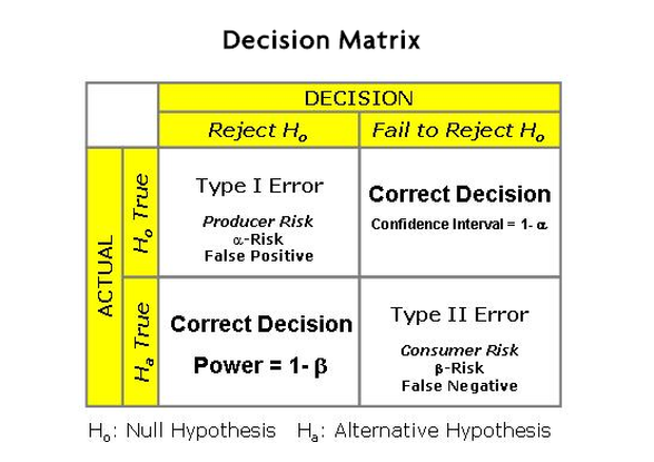
Alpha risk is the risk of incorrectly deciding to reject the null hypothesis. If the confidence interval is 95%, then the alpha risk is 5% or 0.05.
Alpha error is also called False Positive, Producer Risk or Type 1 Error.
Confidence Level = 1 – Alpha
If not otherwise stated then an Alpha risk of 0.05 is assumed, making the confidence level = 95%.
Selecting an Alpha 5% signifies that there is a 5% chance that you were incorrect in rejecting the Null hypothesis.
It’s the amount of risk you are willing to accept of making a Type I error.
Beta risk is the risk that you decide to accept the Null Hypothesis when in fact the reality is that the Alternative Hypothesis is true. In other words, when the decision is made that a difference does not exist when there actually is.
If the power desired is 90% that your testing will correctly identify the Alternative when the Alternative is correct, then the Beta risk is 10%.
The Beta risk being 10% means that there is a 10% chance that the decision will be made that there is no problem, and no action needs to be taken, when in reality there is a problem and some action does need to be taken. Or when the decision is made that a difference does not exist when there actually is a difference.
The Power of a test = 1 – Beta
Beta error is also called False Negative and Type II Error.
The Power is the probability of correctly rejecting the Null Hypothesis.
The Null Hypothesis is technically never proven true. It is “failed to reject” or “rejected”.
“Failed to reject” does not mean accept the null hypothesis since it is established only to be proven false by testing the sample of data.
Consumer’s risk = β = Beta Risk.
Type II error is known as the consumer’s risk because the consumer has accepted a shipment that should be rejected. The shipment contains more than an acceptable number of defectives and will result in more waste or rework than anticipated.
Producer’s risk, α = Alpha Risk
Type I error is referred to as the producer’s risk because the producer made a good lot yet it was rejected.
An operating characteristic curve (OC curve) quantifies these risks on a graph that lets you choose the appropriate sampling plan for the risks you are willing to accept.
2. Use of Takt Time and Cycle Time to calculate number of workers required
TAKT TIME VS CYCLE TIME
Thank you to Lean6Sigma4all and Daniele Giambra for sharing these excellent examples:
Method to calculate the Number of Resources / Workers needed
There could be 2 misunderstandings about how to calculate the Number of Resources that are needed to run a production line or manufacturing cell.
When you implement standard work you have to consider that a Takt Time (TT) is based on customer demand must first be established for the area in question, for example 30 seconds TT, this is equal to set a rate of 120 UPH (Units per Hour).
Therefore; the next question is how many workers are needed in the manufacturing area at this rate?
The answer depends on the total LABOR CONTENT in the area and its relation to demand (TT).
It’s also known as graph of “Takt Time vs Manual Cycle Time”, in many industries.
The more work content, the greater the number of workers that will be required; the less overall work content, the fewer workers that are needed.
Misunderstanding 1:
I have found there is a misunderstanding of Overall Work Content, many people take the Cycle Time complete (Machine + Manual) wich is not right, they must use the “Manual” Overall Work Content (Total Manual Cycle Time)
Here is a PRACTICAL EXAMPLE:
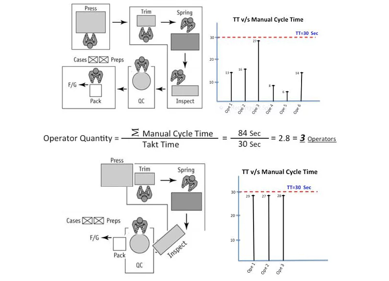
The calculation above shows that is possible to run this Manufacturing Cell with just 3 operators.
Misunderstanding 2:
There is another misunderstanding about the representation of TT, many people don’t understand this concept how to interpret and calculate the Number of Resources when they have operators working in parallel.
For example; when there are operations that are not possible to be separated, the activity must be done from the beginning to the end by one operator at time; and if the cycle time is greater than Takt Time; then you need to use more than one operator to cover the rate needed, this means to have two or more operators working in parallel, for this case the Takt Time must be different.
You should never use the average of those operators as the Manual Work Content, you need represent as it is and make the calculations using other Takt Time equivalent.
Here is a PRACTICAL EXAMPLE:
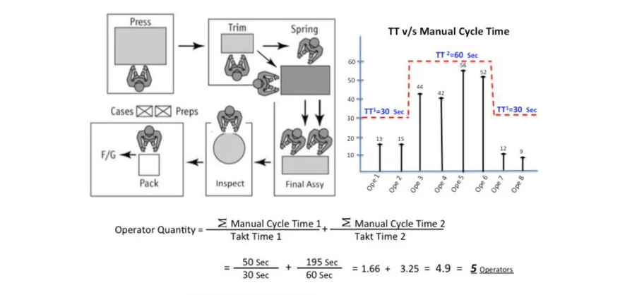
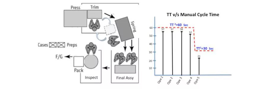
The calculation shows that is possible to run this Manufacturing Cell with just 5 operators; please note that here there is two Takt Times, but do not get confuse at the end the Cell will run at 30 Seconds of Takt Time; equivalent to 120 UPH.
